Observations in the LQ Problem

Let us now extend the reasoning to a description of observations in terms of the pair of variables $x_1 = \log(s_{cp})$ and $x_2 = \log\left( \frac{S_c S_p}{S_W} \right)$ that span the 2D space for the LQ problem. Points in these coordinates are denoted as $\textbf{x} = (x_2, x_1)$. The two-dimensional distribution of growth rates of these coordinates is denoted as $G_{0} (\Delta x_2, \Delta x_1)$, and the region where $x_1 > x_2$ is the two-dimensional plane region $R$ where $\log(s_{cp}) > \log\left( \frac{S_c S_p}{S_W} \right) \Rightarrow s_{cp} > \frac{S_c S_p}{S_W}$, i.e., LQ > 1. The growth cases resulting in the condition LQ > 1 are, in calculus notation:

$$pLQ(\textbf{x}_0) = \iint\limits_{R} G_{0} (\Delta x_2, \Delta x_1) \ ( x_1 > x_2) \ dR$$

This integration would be approximated numerically. A practical way to do so is to store the 2D distribution of growth out of the $\textbf{x}$ coordinates in an array G and the condition $x_1 > x_2$ in another array C of the same shape. In this notation, the numerical integration can simply be:

$$pLQ(\textbf{x}_0) = \text{(G * C).sum() / G.sum()}$$

Before continuing with the strategy for estimation of two-dimensional growth probabilities G, let me emphasize that here we are propagating the volatility of observations and totals into volatility of LQ values.

Volatility and Growth Distributions

First, note that the growth rates of $\log(s_{cp})$ are essentially proportional to the standard deviation $\sigma_{x_1} = \text{std}(\log(s_{cp}))$. This $\sigma_{x_1}$ is larger for smaller entities, but we need to propagate this $\sigma_{x_1}$ to the volatility of LQ values to conclude that smaller entities have higher $\log(LQ)$ jumps. Working with two-dimensional growth distributions as previously described addresses this generally. However, one can take variance in the definition $\log(LQ) := \log(s_{cp}) - (\log(S_c) + \log(S_p) - \log(S_w))$:

$$\text{var}(\Delta \log(LQ)) = \text{var} (\Delta \log(s_{cp}) - \left[ \Delta \log(S_c) + \Delta \log(S_p) - \Delta \log(S_w) \right] ) = \text{var}(\Delta x_1 - \Delta x_2)$$

In empirical settings, jumps in these two terms are largely independent, meaning $\text{cov}(\Delta x_1, \Delta x_2) \approx 0$, so:

$$\text{var}(\Delta \log(LQ)) = \text{var}(\Delta x_1 - \Delta x_2) \approx \text{var}(\Delta x_1) + \text{var}(\Delta x_2)$$ $$\sigma_{\log(LQ)} = \text{std}(\Delta x_1 - \Delta x_2) \approx \sqrt{ \sigma_{x_1} + \sigma_{x_2} }$$

Volatility Decay with Size

It turns out that $\text{var}(\Delta x_1)$ and $\text{var}(\Delta x_2)$ are functions of $x_1$ and $x_2$, respectively. These volatilities are plotted in Figure 1. Larger nominal values fluctuate less in relative terms than smaller values, consistent with findings from Stanley et al. and others studying volatility decay with size. This dependence means that $\text{var}(\Delta \log(LQ))$ is a function of $x_1, x_2$, i.e., the sizes.

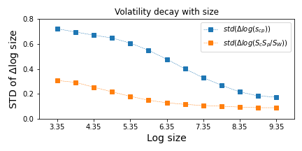
Volatility versus size. Larger observations fluctuate less and are less likely to traverse a given gap in LQ levels. The standard deviation in these plots is the width of the axis of ellipses in the subsequent figures.

Ellipse Representation of Volatility

This expression of volatility of $\Delta \log(LQ)$ is linked to equations of ellipses. Using the notation $\sigma^2_{\log(LQ)} = \sigma^2_{x_1} + \sigma^2_{x_2}$ for variances of the jumps ($\Delta$), recall the equation of an ellipse centered at the origin is $k^2 = (x/a)^2 + (y/b)^2$ where $a$, $b$ are the semi-minor and major axes, and $k$ is a measure of ellipse size. Associating the ellipse axes with the width of jumps in $x_1$, $x_2$, the magnitude of $\Delta \log(LQ) = \Delta x_1 - \Delta x_2$ jumps is determined. These are the jumps in $\log(LQ)$, in the sense that $\log(LQ)_{t+1} = \log(LQ)_t + \Delta \log(LQ)$. See Figure 2 for a schematic diagram.

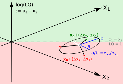
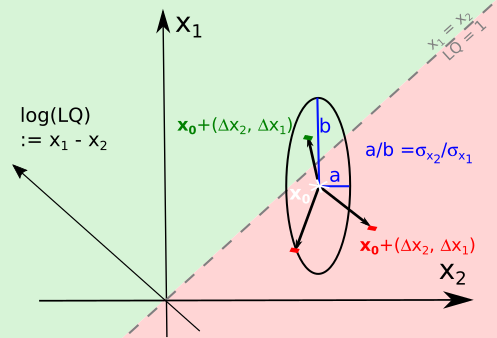
Scheme of jumps in observations after a time step. Using size factor $y_2 = (x_1 + x_2)/2$ and log(LQ) as axes (left) and observed and expected sizes $x_2, x_2$ as axes (right). The green regions are those where $LQ > 1$. The initial point $\bm{x_0}$ is shown with a white star. Around it, three purported jumps after a timestep are drawn. The ellipses indicate how far jumps are expected to stretch, in the directions $x_1$ and $x_2$ and thus in any other direction given by a combination of those.

Finally, even after characterizing the widths of the jumps in $x_1$, $x_2$, and thus $\log(LQ)$, there remains a step to translate it into chances of surpassing the $LQ = 1$ threshold (pLQ). For that, let us return to our core goal of explaining pLQ by means of growth distributions. We need to count all cases where jumps have let $\log(LQ) > 1$.