pLQ as Predictor for Diversification

pLQ as a Predictor for Diversification

In this section, we explore how the pLQ (probability of Location Quotient) integrates into a framework for predicting diversification. We compare a fixed effects regression, inspired by Hausmann's approach, using both the binary $LQ > 1$ and pLQ. The second independent variable is proximity $w$ .

Proximities are computed using the same operations but start from $LQ > 1$ and pLQ matrices respectively. These variables coincide for most practical purposes.

The regression equation includes dummies for each country-product and time period fixed effects:

y_{it} = \alpha +\beta_1 x_{it} + \beta_2 w_{it} + \pi_{i} \delta_{i} + \pi_{t} \delta_{t} + \epsilon_{it}

$i$ : Represents a country-product.
$y_{it}$ : Dependent variable indicating if $LQ > 1$ for country-product $i$ at time $t+1$ .
$\alpha$ : Intercept term.
$x_{it}$ : Refers to either pLQ or binary $LQ > 1$ for country-product $i$ at time $t$ .
$\delta$ : Dummies for country-product and time step.
$\pi$ : Corresponding coefficients.
$\epsilon_{it}$ : Error term.

To manage the numerous dummies, we apply the within transformation:

y^{*} = y -\bar{y_i} - \bar{y_t} + \bar{\bar{y}}

This transformation 'sweeps' the $\pi_{i}$ and $\pi_{t}$ effects, allowing us to fit the within estimators $\tilde \beta$ using OLS:

y^{*}_{it} = \tilde \beta_1 x^{*}_{it} + \tilde \beta_2 w^{*}_{it} + \epsilon^{*}_{it}

The results are summarized below:

	Fitted Coefficients (1)	Fitted Coefficients (2)
Binary LQ ( $\beta_1$ )	0.756 $\ast$
	(0.001)
pLQ ( $\beta_1$ )		0.986 $\ast$
		(0.001)
Density ( $\beta_2$ )	0.065 $\ast$	0.021 $\ast$
	(0.001)	(0.001)
Adj. R-squared	0.682	0.623
No. of Observations	1,404,542	1,404,556

Note: Statistically significant at the 0.01% level.

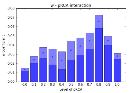
We also examine if the role of density varies for different levels of pLQ. By applying a simple interaction with a dummy indicating the level of pLQ, the fitting equation becomes:

y^{*}_{it} = \tilde \beta_1 x^{*}_{it} + \tilde \gamma_k w^{*}_{it} \delta_{k} + \epsilon^{*}_{it}, \ \ k = 0, ..., 10

The mean value and 2.5% - 97.5% confidence interval for all density coefficients $\gamma_k$ are plotted in the figure below. This suggests that density plays a more significant role for products slightly above the $LQ = 1$ threshold.

Interaction Coefficients

A possible integration of this framework into similar regressions could involve assigning a value of 0.5 to indicate if a country exports a product with an intermediate level of LQ.