Firm Level Fluctuations

Firm Level Fluctuations

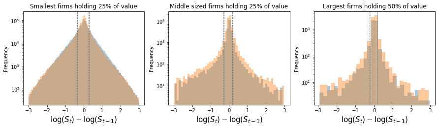
If firm sales are expressed in logs, it is natural to describe their dynamics as changes in log levels. Figure 1 illustrates the observed distribution of year-on-year log differences. The plots depict growth rates for:

• The smallest firms concentrating up to 25% of the value
• Intermediate size firms accounting for the next 25% of sold value
• The largest firms concentrating 50% of the value

Results for exports and imports largely overlap in each of the plots. The scale is log-log, so that:

• A double exponential (Laplace) distribution would appear as $\sim -|x|$
• Normally distributed log shocks would appear as $\sim - x^2$
• For large firms, we observe $\sim -|x|^c$ with $0 < c < 1$

We see nearly symmetric fluctuations.

Very importantly, when computing total sales by firms $k$ at time $t$, we need to consider the terms in $\sum S_{kt}$. This can be reconstructed by knowing the initial value $S_{k0}$ and accumulating the log shocks up to $t$. This method is known as the growth rates accumulation approach. However, reconstructing the time series of levels of a firm solely from the general distribution of log differences would be a mistake because it ignores existing autocorrelation structures. In most empirical settings, there is a mild negative one-step autocorrelation of log shocks, meaning growth events are more likely followed by shrinkage events and vice versa.

To avoid these complications, we can express the information of firm sales levels as deviations from a stationary (or average) value. In this case, we do not need to accumulate a time series of log growth rates anymore. This is observed directly from the empirical data (Figure 2). Deriving analytical expressions for these distributions is not straightforward, but unnecessary.

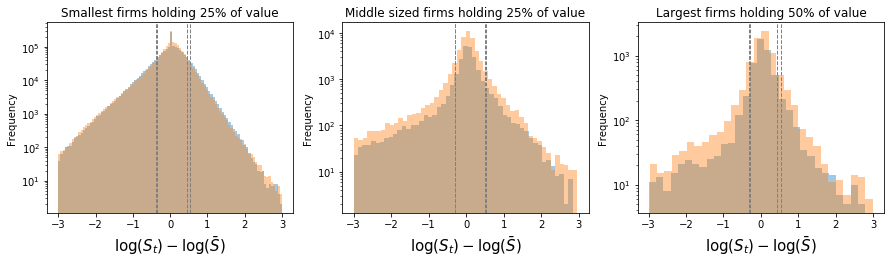
The values illustrated in Figure 2 are termed fluctuations, distinguishing them from log jumps shown by agents (as in growth rates). Consider these distributions ($D(.)$) as the large numbers limit distribution of deviations of a firm from its average value $\bar s$. To sum the value sold by this firm over time, one would need to sum the values $\bar s 10^{D(.)}$. Similarly, if $D(.)$ is the limit distribution of deviations for a population of firms at any given time step from their mean $\bar s$, then summing $\bar s 10^{D(.)}$ gives total sales at each time step.

Expressing the information on firm levels over time as fluctuations has a dual advantage: it avoids the problem of accumulation of autocorrelated time series and their powers are exactly what one needs to sum to obtain aggregates.

The most important feature of firm-level fluctuations is their natural adaptation to a description of the type $10^{D(.)}$, where $D(\cdot)$ is usually a mixture of Gaussians. This characteristic is crucial as it determines the formal path for aggregating them.